Volleyball R package: `volleystat`
Open Source Data: Overview
Datasets and variables
The volleystat package is an open-source statistics repository for the Men & Female German Bundesliga Volleyball League (1st Division) created by Viktor Bozhinov. The package contain the following datasets/dataframes, including: matches, matchstats, match_addresses, players, sets, staff, and team_addresses.
For example, here are some of the variables included in the players and sets dataframes:
| season_id | league_gender | team_id | team_name | lastname | firstname | height | gender | birthdate | shirt_number | position | nationality | player_id |
|---|---|---|---|---|---|---|---|---|---|---|---|---|
| 1617 | Men | 1001 | Solingen Volleys | Bevers | Lennart | 179 | male | 1993-07-10 | 10 | Libero | Germany | 10 |
| 1617 | Men | 1001 | Solingen Volleys | den Boer | Huib | 191 | male | 1981-11-11 | 2 | Setter | Netherlands | 2 |
| 1617 | Men | 1001 | Solingen Volleys | Gies | Oliver | 197 | male | 1985-06-28 | 3 | Outside spiker | Germany | 3 |
| 1617 | Men | 1001 | Solingen Volleys | Gosmann | Christian | 191 | male | 1992-07-02 | 6 | Universal | Germany | 6 |
| 1617 | Men | 1001 | Solingen Volleys | Horn | Maximilian | 188 | male | 1996-08-07 | 4 | Setter | Germany | 4 |
| league_gender | season_id | match_id | match | team_id | team_name | set | set_duration | pt_set |
|---|---|---|---|---|---|---|---|---|
| Women | 1314 | 2003 | home | 2001 | Allianz MTV Stuttgart | 1 | 23 | 18 |
| Women | 1314 | 2002 | home | 2002 | Dresdner SC | 1 | 23 | 25 |
| Women | 1314 | 2004 | home | 2008 | USC Münster | 1 | 27 | 22 |
| Women | 1314 | 2001 | home | 2005 | Rote Raben Vilsbiburg | 1 | 27 | 26 |
| Women | 1314 | 2005 | home | 2009 | VC Wiesbaden | 1 | 19 | 25 |
Data source
The data was collected from the official Bundesliga Volleyball website. It covers the games played from the 2013/14 to the 2018/19 season.
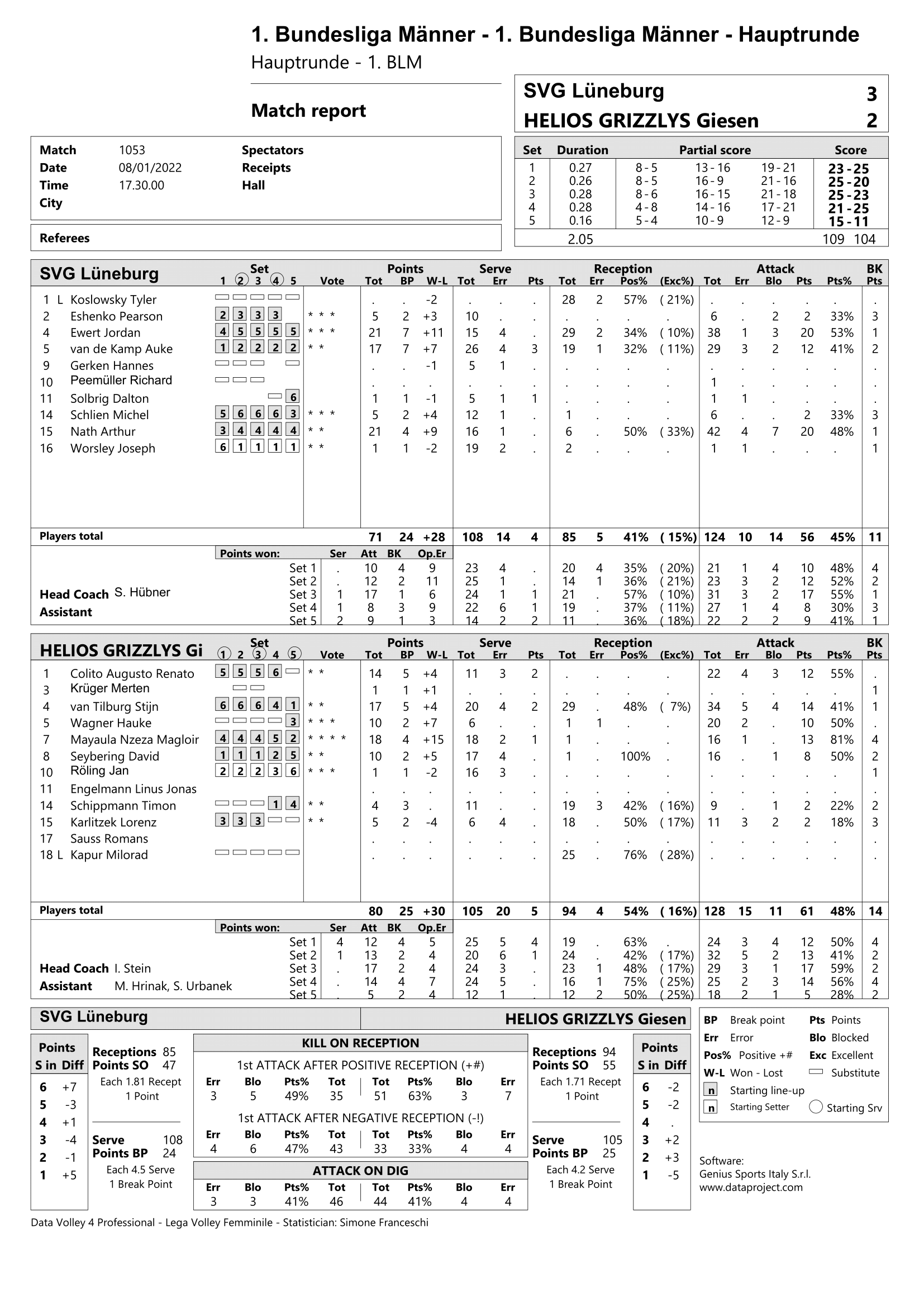
Specfically, the in-game match statistics were collected/scraped directly from official game reports using the tabulizer package:
Example game report:
Accessing the data
Accessing the data is quite straightforward, as the datasets are directly accessible from the volleystat package itself. Therefore you can either access the dataset directly:
1
2
3
4
volleystat::matches
volleystat::matchstats
volleystat::players
# and so on...
Unfortunately, one limitation of this package is that the data is scraped directly from the game reports (.pdf), therefore, the package will only be updated with new data once the package creator manually scrapes recent games and uploads them.
Possible research questions
As the volleystat package contains multiple variables, there are multiple research questions that can be produced, for example:
- Is there a relationship between longer match/set times and player metrics?
- Using player metrics from the matchstats dataset and
match_duration/set_durationfrom the matches/sets datasets respectively, we can discover any correlations for specific player metrics.
- Using player metrics from the matchstats dataset and
- What player metrics best predict match outcome?
- We can create a new variable, match outcome, which can be used as a dependent variable in a predictive model using player metrics from matchstats as our predictor variables.
- Does playing at home, time of match and spectator count influence match outcome?
- Variables for home or away, match time and spectator count can be extracted from the matches dataset, which can then be compared to a match outcome variable (created via data manipulation).
Unfortunately, the volleystat package does not include hawkeye-like data containing x,y co-ordinates of the ball, nor any LPS/Optical tracking data for player position on the court.
Not having access to this data makes it difficult/impossible to analyse parts of the games such as:
- setter choice/selection
- spike choice/selection
- service choice/selection
- defence formation on attack
Visualisations
This section will demonstrate what types of visualisations can be created through manipulation of data obtained from the volleystat package (all visualisations were made with the package ggplot2). The code for initial data wrangling performed can be viewed below.
Code: initial data wrangling
1
2
3
4
5
6
7
8
9
10
11
12
13
14
15
16
17
18
19
20
21
22
23
24
25
26
27
28
29
30
31
32
33
34
35
36
# Load required libraries
library(volleystat)
library(tidyverse)
library(kableExtra)
library(ggbump)
library(ggsci)

# Join matchstats & team_adresses from volleystat to know which team played which games
match_team_join <- left_join(volleystat::matchstats,
                             volleystat::team_adresses,
                             by = c('team_id' = 'team_id',
                                    'season_id' = 'season_id')
) %>%
  select(-c(league_gender.y, gym_adress, max_spectators, lon, lat))

# Calculate team statistics for each team grouped by season
team_summary_stats <- match_team_join %>%
  group_by(team_name, season_id, league_gender.x) %>%
  summarise(pt_total = sum(pt_tot), # not using summarise(across) as I want to rename columns
            serv_total = sum(serv_tot),
            aces = sum(serv_pt),
            serv_error = sum(serv_err),
            rec_total = sum(rec_tot),
            rec_error = sum(rec_err),
            att_total = sum(att_tot),
            att_error = sum(att_err),
            att_block = sum(att_blo),
            att_pt = sum(att_pt),
            block_pt = sum(blo_pt)) %>%
  mutate(team_name_abrv = abbreviate(team_name), # create abbreviated team_names for data viz
         season_id = case_when(season_id == 1314 ~ '2013/14',
                               season_id == 1415 ~ '2014/15',
                               season_id == 1516 ~ '2015/16',
                               season_id == 1617 ~ '2016/17',
                               season_id == 1718 ~ '2017/18',
                               season_id == 1819 ~ '2018/19'))
1
2
## `summarise()` has grouped output by 'team_name', 'season_id'. You can override
## using the `.groups` argument.
1
2
3
4
5
6
7
8
9
10
11
         #season_id = str_replace(season_id, '(\\d)(\\d{2}$)', '\\1/\\2')) # season xxyy to xx/yy

# Convert team_summary_stats to long format for data viz
team_stats_long <- team_summary_stats %>%
  pivot_longer(cols = pt_total:block_pt,
               names_to = 'pt_metrics')

# Calculating season averages for each metric
season_avg_long <- team_stats_long %>%
  group_by(season_id, pt_metrics, league_gender.x) %>%
  summarise(avg = round(mean(value)))
1
2
## `summarise()` has grouped output by 'season_id', 'pt_metrics'. You can override
## using the `.groups` argument.
Additionally to add some context, a table of metric definitions has been provided below.
| Metrics | Descriptions |
|---|---|
| pt_total | Total points scored |
| serv_total | Total number of serves |
| aces | Total number of service aces |
| serv_error | Total number of service errors |
| rec_total | Total number of receptions from serve |
| rec_error | Total number of receptions errors |
| att_total | Total number of attacks/spikes |
| att_error | Total number of attacking errors |
| att_block | Total number of blocks |
| att_pt | Total number of successful attacks |
| block_pt | Total number of successful blocks |
Men’s League
Here is a visualisation that looks at the top 3 and bottom 3 performing teams of the Men’s Bundeliga 18/19 Volleyball Competition.
Code: additional data wrangling
1
2
3
4
5
6
7
8
9
10
11
12
13
14
15
16
17
18
19
20
21
22
23
24
25
26
27
28
29
30
top3_bottom3_1819_men <- team_stats_long %>%
  filter(league_gender.x == 'Men',
         team_name %in% c('Berlin Recycling Volleys',
                          'VfB Friedrichshafen',
                          'Hypo Tirol AlpenVolleys Haching',
                          'VCO Berlin',
                          'TV Rottenburg',
                          'Helios Grizzlys Giesen'),
         season_id =='2018/19') %>%
  # Add final seed to name for legend
  mutate(team_name = case_when(team_name == 'Berlin Recycling Volleys' ~ 'Berlin Recycling Volleys (1)',
                               team_name == 'VfB Friedrichshafen' ~ 'VfB Friedrichshafen (2)',
                               team_name == 'Hypo Tirol AlpenVolleys Haching' ~ 'Hypo Tirol AlpenVolleys Haching (3)',
                               team_name == 'Helios Grizzlys Giesen' ~ 'Helios Grizzlys Giesen (10)',
                               team_name == 'TV Rottenburg' ~ 'TV Rottenburg (11)',
                               team_name == 'VCO Berlin' ~ 'VCO Berlin (12)'),
         # Re-level for ordering in legend, weird ordering as legend is at the bottom
         team_name = factor(team_name, levels = c('Berlin Recycling Volleys (1)',
                                                  'Helios Grizzlys Giesen (10)',
                                                  'VfB Friedrichshafen (2)',
                                                  'TV Rottenburg (11)',
                                                  'Hypo Tirol AlpenVolleys Haching (3)',
                                                  'VCO Berlin (12)')),
         # Also re-level the abbreviated team names for the x-axis
         team_name_abrv = factor(team_name_abrv, levels = c('BrRV',
                                                            'VfBF',
                                                            'HTAH',
                                                            'HlGG',
                                                            'TVRt',
                                                            'VCOB')))
Code: data visualisations
1
2
3
4
5
6
7
8
9
10
11
12
13
14
15
16
17
18
19
ggplot(top3_bottom3_1819_men, aes(x = team_name_abrv, y = value, fill = team_name)) +
  geom_col() +
  facet_wrap(~pt_metrics, scales = 'free_y') +
  geom_hline(data = season_avg_long %>% filter(league_gender.x == 'Men', season_id == '2018/19'),
             aes(yintercept = avg, linetype = 'League Average'), linewidth = 0.7, col = '#54D421') +
  theme_bw() +
  theme(panel.grid.major.x = element_blank(),
        legend.position = 'bottom',
        legend.text = element_text(size = 11),
        legend.title = element_text(size = 13),
        axis.text = element_text(colour = 'black'),
        panel.background = element_rect(fill = '#f1f1f1')) +
  labs(fill = 'Team',
       linetype = '') + # change legend title
  ggtitle('Comparison of top 3 and bottom 3 teams for the 18/19 season, w/ league avg.') +
  ylab('Quantity') +
  xlab('') +
  scale_fill_manual(values = c("#375681", "#db571a", "#4972ab", "#E76E36", "#7092c2", "#EC895B")) +
  scale_linetype_manual(values = 5)
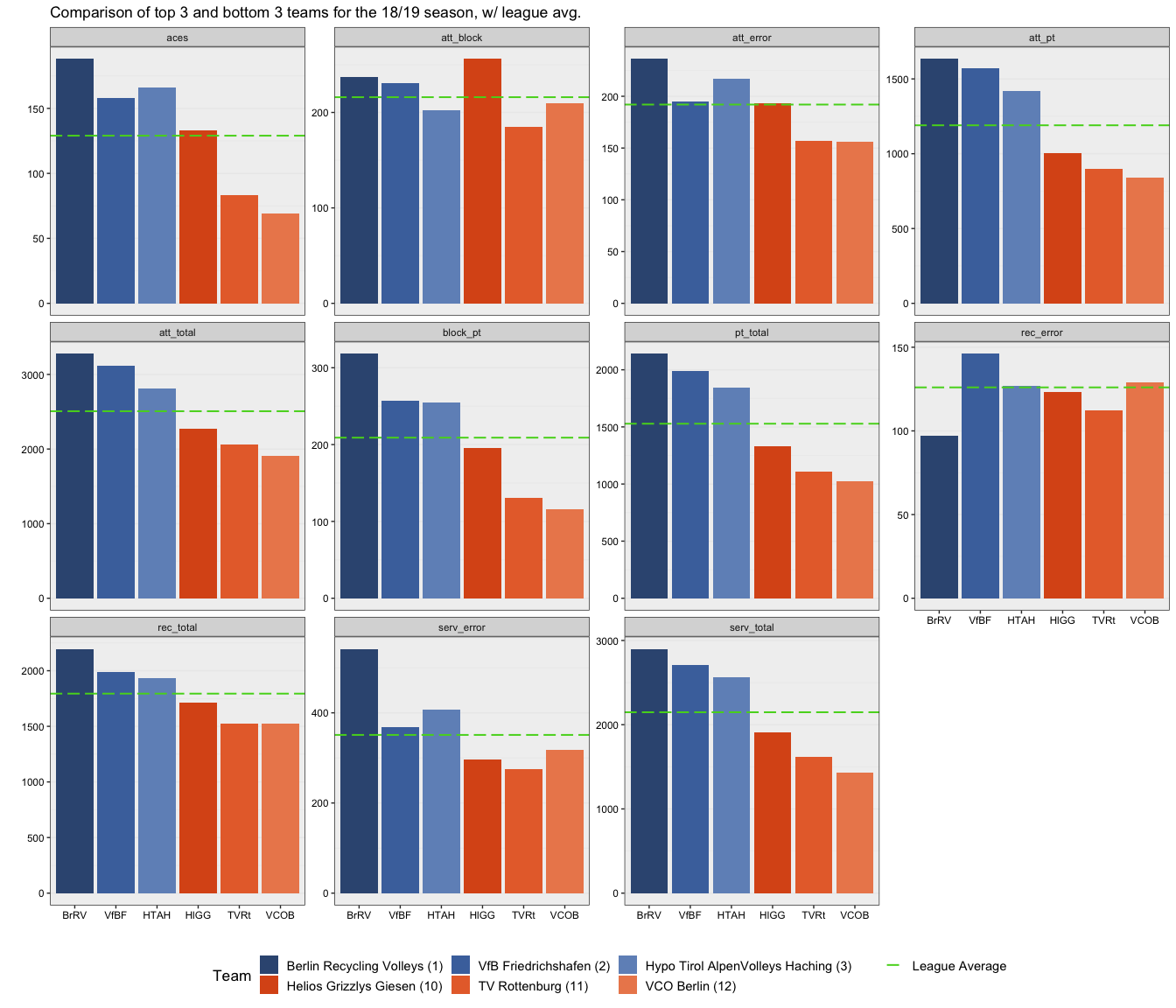
For nearly all of the metrics, the top 3 performing teams were above the season average, while the bottom performing teams were for the most part under the league average, which is mostly to be expected. This visual might also give some insight to coaches on the importance of some metrics compared to others. For instance seeing a possible correlation between aces and serv_error where the top 3 teams are taking more risks serving, hence the higher serv_error rates, but also have a higher number of aces. This may be something the bottom 3 teams could incoroporate into their game to try and be more successful.
Women’s League
I thought I would change it up for the women’s league and explore the service metrics across all the seasons.
Code: additional data wrangling
1
2
3
4
5
6
7
8
9
10
11
12
serve_metrics_13to19 <- team_stats_long %>%
  filter(league_gender.x == 'Women',
         pt_metrics %in% c('serv_total', 'aces', 'serv_error'),
         team_name_abrv %in% c('AMTS', # filter to only have teams across all seasons
                               'DrSC',
                               'LiBA',
                               'RtRV',
                               'SCPt',
                               'SSCS',
                               'USCM',
                               'VCWs',
                               'VIIT'))
Code: data visualisations
1
2
3
4
5
6
7
8
9
10
11
12
13
14
15
16
ggplot(serve_metrics_13to19,aes(x = season_id, y = value, col = team_name)) +
  geom_bump(aes(group = team_name), linewidth = 0.7) + # have to add group = team_name when x-axis categorical
  geom_point(size = 1) +
  facet_wrap(~pt_metrics, scales = 'free_y') +
  theme_bw() +
  theme(panel.grid.minor.x = element_blank(),
        legend.position = 'bottom',
        legend.text = element_text(size = 11),
        legend.title = element_text(size = 13),
        axis.text = element_text(colour = 'black'),
        panel.background = element_rect(fill = '#f1f1f1')) +
  labs(col = 'Team') +
  ggtitle('Service metric comparison for Womens Bundesliga from 2013/14 to 2018/19 ') +
  ylab('Quantity') +
  xlab('Season') +
  scale_color_d3()
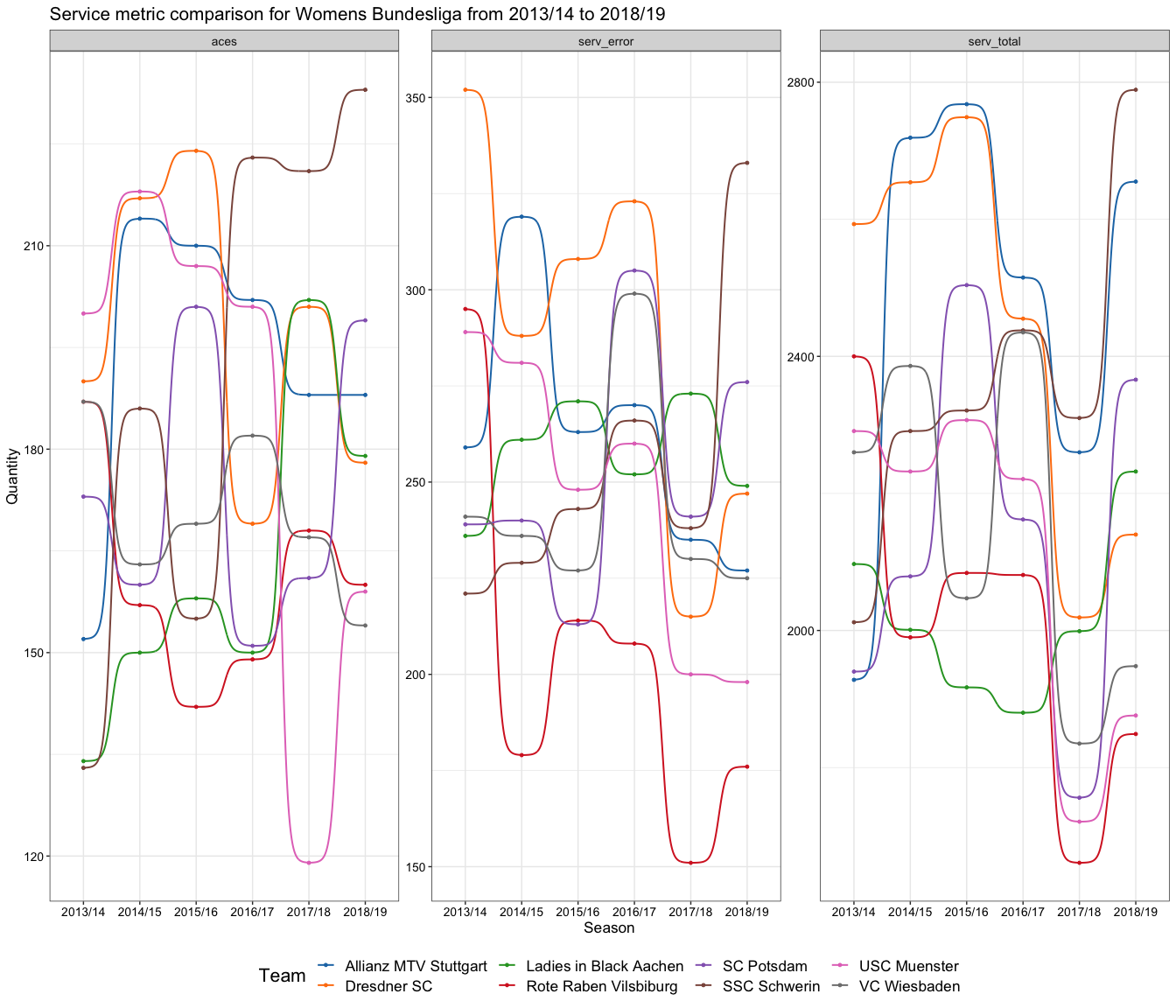
As for the women’s visualisation, all the teams are quite varied over the various seasons, which is somewhat expected as player transfers are a thing. To add a little more context I’ve also added a table below that shows where each team placed on the final ladder per season (only decided to keep teams in this graph in the table, which explains the missing values).
| 2013/14 | 2014/15 | 2015/16 | 2016/17 | 2017/18 | 2018/19 | |
|---|---|---|---|---|---|---|
| 1st | Dresdner SC | Dresdner SC | Dresdner SC | SSC Schwerin | Allianz MTV Stuttgart | Allianz MTV Stuttgart |
| 2nd | VC Wiesbaden | Allianz MTV Stuttgart | SSC Schwerin | Allianz MTV Stuttgart | Dresdner SC | SSC Schwerin |
| 3rd | Rote Raben Vilsbiburg | SSC Schwerin | Allianz MTV Stuttgart | Dresdner SC | SSC Schwerin | Dresdner SC |
| 4th | Ladies in Black Aachen | VC Wiesbaden | USC Muenster | SC Potsdam | VC Wiesbaden | SC Potsdam |
| 5th | SSC Schwerin | SC Potsdam | VC Wiesbaden | VC Wiesbaden | Ladies in Black Aachen | Rote Raben Vilsbiburg |
| 6th | SC Potsdam | Ladies in Black Aachen | Rote Raben Vilsbiburg | Rote Raben Vilsbiburg | USC Muenster | Ladies in Black Aachen |
| 7th | USC Muenster | USC Muenster | SC Potsdam | USC Muenster | SC Potsdam | USC Muenster |
| 8th | - | Rote Raben Vilsbiburg | - | Ladies in Black Aachen | Rote Raben Vilsbiburg | VC Wiesbaden |
| 9th | Allianz MTV Stuttgart | - | - | - | - | - |
| 10th | - | - | Ladies in Black Aachen | - | - | - |
| 11th | - | - | - | - | - | - |
| 12th | - | - | - | - | - | - |
| 13th | - | - | - | - | - | - |